Transformers (State-of-the-art Natural Language Processing).
Part 1/3 of Transformers vs Google QUEST Q&A Labeling (Kaggle top 5%).

This is a 3 part series where we will be going through Transformers, BERT, and a hands-on Kaggle challenge — Google QUEST Q&A Labeling to see Transformers in action (top 4.4% on the leaderboard).
In this part (1/3) we will be looking at how Transformers became state-of-the-art in various modern natural language processing tasks and their working.
The Transformer is a deep learning model proposed in the paper Attention is All You Need by researchers at Google and the University of Toronto in 2017, used primarily in the field of natural language processing (NLP).
Like recurrent neural networks (RNNs), Transformers are designed to handle sequential data, such as natural language, for tasks such as translation and text summarization. However, unlike RNNs, Transformers do not require that the sequential data be processed in the order. For example, if the input data is a natural language sentence, the Transformer does not need to process the beginning of it before the end. Due to this feature, the Transformer allows for much more parallelization than RNNs and therefore reduced training times.
Transformers were designed around the concept of attention mechanism which was designed to help memorize long source sentences in neural machine translation.
Sounds cool right? Let’s take a look under the hood and see how things work.

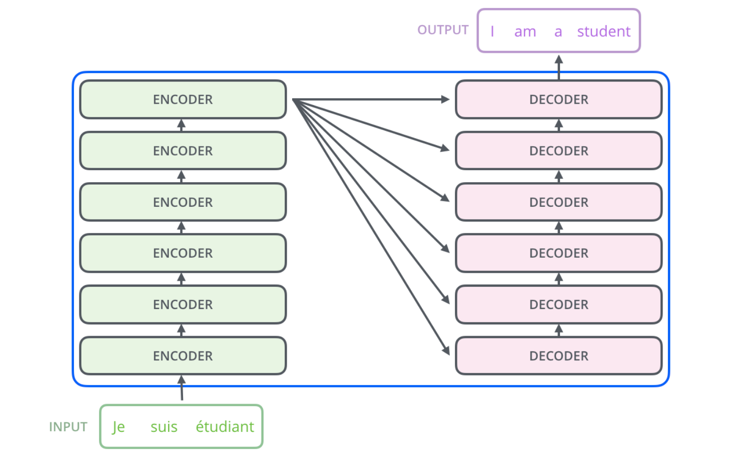
Transformers are based on an encoder-decoder architecture that comprises of encoders which consists of a set of encoding layers that processes the input iteratively one layer after another and decoders that consists of a set of decoding layers that does the same thing to the output of the encoder.
So, when we pass a sentence into a transformer, it is embedded and passed into a stack of encoders. The output from the final encoder is then passed into each decoder block in the decoder stack. The decoder stack then generates the output.
All the encoder blocks in the transformer are identical and similarly, all the decoder blocks in the transformer are identical.
This was a very high-level representation of a transformer and it wouldn’t probably make much sense when understanding how transformers are so efficient in modern NLP tasks.
Don’t worry, to make things clearer, we will go through the internals of an encoder and decoder cell now…
Encoder
The encoder has 2 parts, self-attention, and a feed-forward neural network.
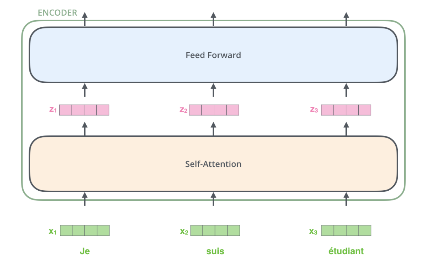
The encoder’s inputs first flow through a self-attention layer — a layer that helps the encoder look at other words in the input sentence as it encodes a specific word. Basically for each input word ‘x’ the self-attention layer generates a vector Z such that it takes all the input words (x1, x2, x3, …, xn) into the picture before generating Z. I’ll come to why it takes all the input word’s embedding into the picture and how it generates Z later in this blog but for now, just remember these brief high-level summarizations of the subcomponents of an encoder.
The outputs of the self-attention layer are fed to a feed-forward neural network. The feed-forward neural network generates an output for each input Z and the output from the feed-forward neural network is passed into the next encoder block’s self-attention layer and so on.
Now that we have an idea of what all is inside an encoder, let’s understand the tensor operations happening inside each component.
First comes the input:
We know that transformers are used for NLP tasks so the data we deal with is usually a corpus of sentences, but since machine learning algorithms are all about matrix operations, we first need to convert the human-readable sentences into a machine-readable format (numbers). To convert the sentences into numbers, we use ‘word embeddings’. This step is simple, each word in a sentence is represented as an n-dimensional vector (n is usually 512) and for transformers, we typically use GloVe embedding representation of words. There is also something called positional encoding that is applied to these embedding but I’ll come to it later. Once we have the embedding for each input word, we pass these embedding simultaneously to the self-attention layer.
The training parameters of self-attention layer:
Different layers have different learning parameters eg. a Dense layer has weights and bias, a Convolutional layer has kernels as the learning parameters similarly in the self-attention layer, we have 4 learning parameters:
- Query matrix: Wq
- Key matrix: Wk
- Value matrix: Wv
- Output matrix: Wo (this is not the output matrix but a trainable parameter that generates the final output of the self-attention layer Z).
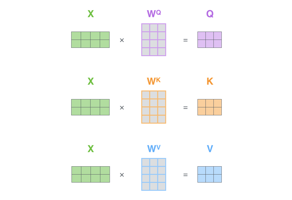
The first 3 trainable parameters have a special purpose, they are used for generating 3 new parameters:
- Query: Q
- Key: K
- Value: V which are later used for generating output Z from input x, let’s see how-
Some points to keep in mind are:
- The input tensor x has n-rows and m-columns where n is the number of input words and m is the vector size of each word i.e. 512.
- The output tensors Q, K, V, and Z have n-rows and dk-columns where n is the number of input words and dk is 64. The values of m and dk are no random values but were found to work the best by researchers who came up with this architecture.
After calculating the 3 parameters Q, K, V as mentioned above, the self-attention layer then calculates scores, a vector for each of the input words.
Dot-product attention:
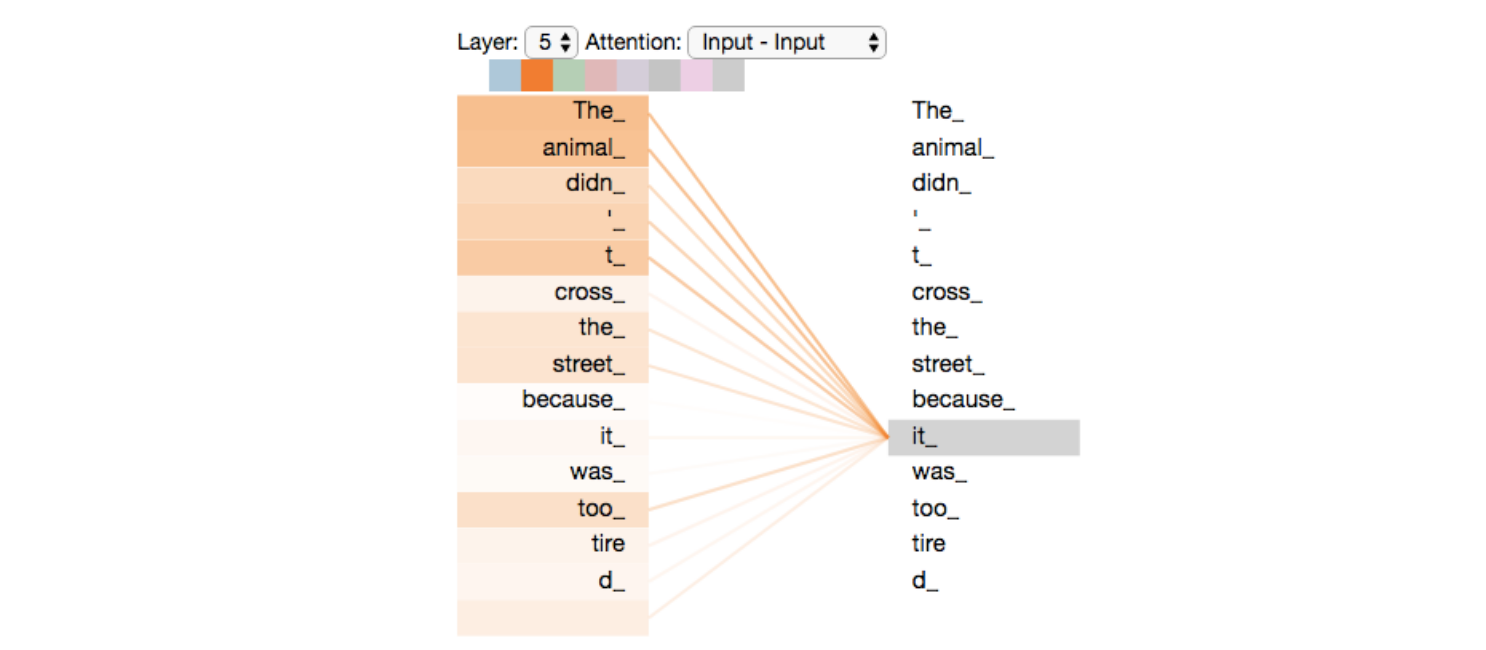
The next step in the self-attention layer is to calculate the value of the vector score corresponding to each input word. This score calculation is one of the most crucial steps that bring the attention mechanism to life (well… not literally). The vector score has a size of n where n is the number of input words and each element of this vector is a number that tells how much does the word that it corresponds to contributes to the current word. Let’s consider an example to get the intuition- “The animal didn’t cross the street because it was too tired” In the above sentence, the word it refers to the animal and not the road. For us, this is pretty simple to grasp but not for a machine with no attention, because we know how grammar works and we’ve developed a sense that it will be referring to animal more than words like cross or road. This sense of grammar comes to transformers after training but the fact that for a given word, it considers all the words in the input and then has the ability to select the one that it thinks contributes the most is what the attention mechanism is about. For the above sentence, the score vector generated for the word it will have 11 numbers, each corresponding to a word in the input sentence. For a well-trained model, this score vector will have larger numbers at positions 2 and 8 because the words at 2(animal) and 8(it) contribute the most to it. It may look something like: [2, 60, 4, 5, 3, 8, 5, 90, 7, 6, 3] Notice that the values at positions 2 and 8 are greater than the values at other positions.
Let’s see how these scores are generated in the self-attention layer.
Till now, for each word, we have Q, K, V vectors. To generate the score vector, we use something called the dot-product attention where we take a dot product between the Q and the K vectors to generate the score. The value of Q is corresponding to the query of the word for which we are calculating the score, in the above example, the word was it whereas there are n values of K, each corresponding to the key vector of the input words.
So, if we want to generate the scores for the word it:
-
We take the query vector of it: Q
-
We take the key vectors of the input sentences: K1, K2, K3, …, Kn.
-
We take a dot product between Q and K’s and obtain n scores.
After calculating the scores, we kind of normalize the scores by dividing them by squared root of (dk) which was the column-dimension of vectors Q, K, V. This step was mandatory because the creators of the transformer found that normalizing the scores by sqrt. of dk gives better results.
After normalizing the score vectors, we encode them using softmax function such that the output is proportional to the original scores but all the values sum up to 1.
Once we have the ‘softmaxed’ scores ready, we simply multiply each score element with the value vector V corresponding to it, such that we get n value vectors V after this operation: [V1, V2, V3, …, Vn]. Now to obtain the output Z of the self-attention, we simply add all the n value vectors.


The above diagrams illustrate the steps of the self-attention layer.
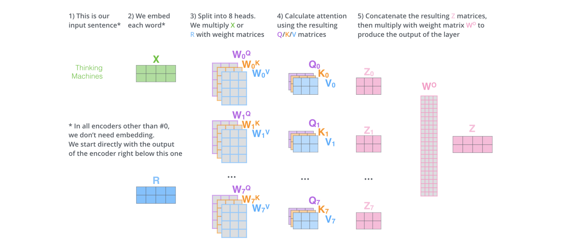
Multi-head Attention:
Now that we know how an attention-head works, and how amazing it is there is a catch to it. A single attention-head can sometimes miss some of the words in input that contribute most to the spotlight word, like in the example before, sometimes the attention head may fail to pay attention to the word animal while predicting the word it and this may cause problems. To tackle this issue, instead of just a single attention-head, we use multiple attention-heads, each working in a similar manner. This idea helps us to reduce the error or miscalculation by any single attention head. This is also referred to as multi-head attention.

In the transformers, multi-head attention typically uses 8 attention heads.
Now notice that the output of a single attention-head was of 64 dimensions, but if we use multi-head attention, we will get 8 such 64-dimensional vectors as output.

Turns out there is a final trainable parameter Output matrix Wo that I mentioned before that comes into play here.
In the final layer of the self-attention, all the output [Z0, Z1, Z2,…, Z7] are concatenated and multiplied with Wo such that the final output Z is of a dimension 64.
Below is the diagram to show all the steps discussed above:
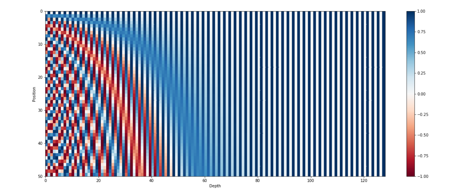
Positional encoding:
Remember in first comes the input section I mentioned positional encoding, let’s see what are they and how they help. The problem with our current awesome transformer is that it does not take the position of the input words into account. Unlike RNN where we had timesteps to denote which word comes before and after, in transformers since the words are fed simultaneously, we need some kind of positional encoding that defines which word comes after which. Positional encoding comes to our rescue as it gives the input embedding a sense of position, we first generate the position embeddings for each of the input words and these position embeddings are then added to the word embeddings of the respective words to generate embeddings with a time signal.
There were many proposed method for generating the positional embeddings like one-hot encoded vectors or binary encoding but what the researchers found to work the best was using the equations below to generate the embeddings:

When we plot the 128-dimensional positional encoding for a sentence with a maximum length of 50, it looks something like:
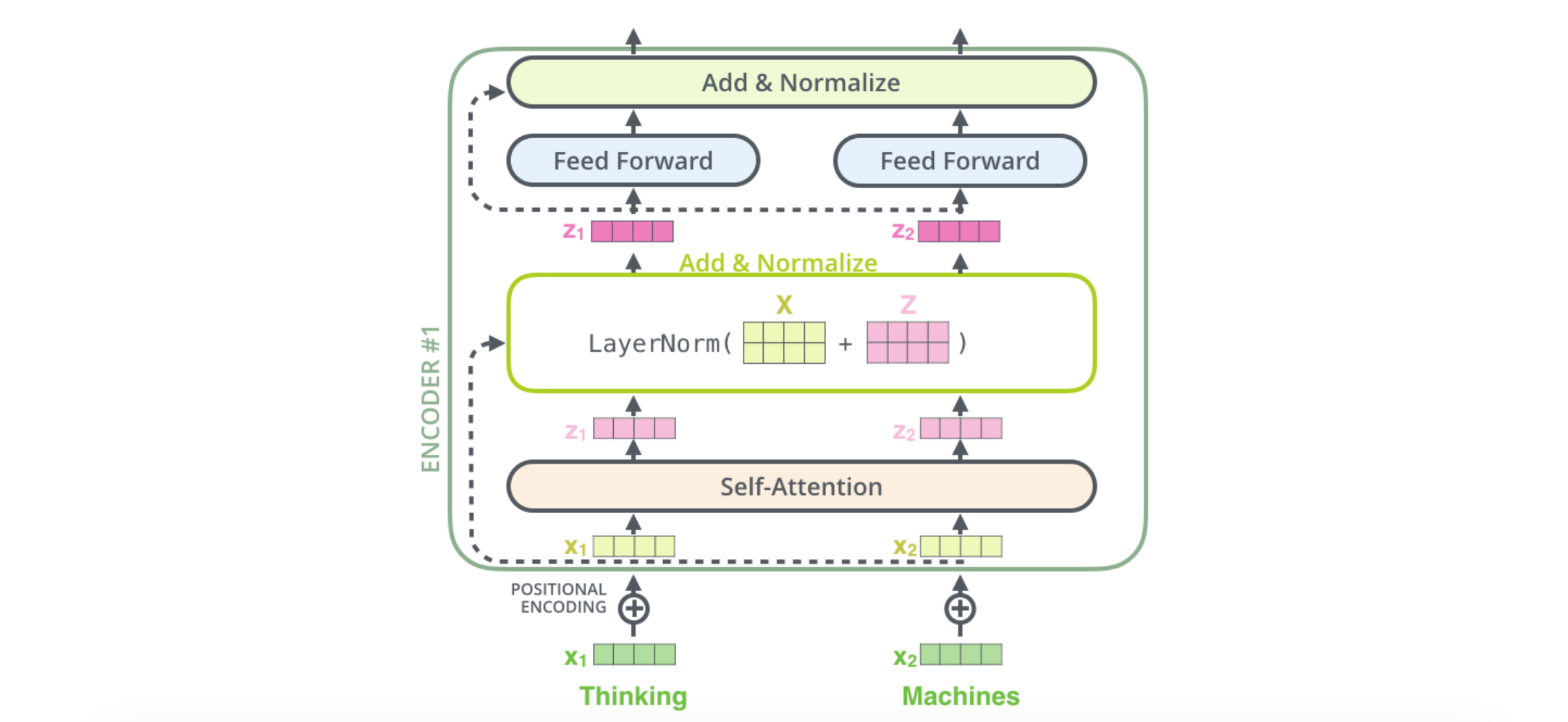
Residual connections:
Finally, there is one more improvisation added to the encoders known as residual connections or skip connections which allow the output from the previous layer to bypass layers in between. It helps in deep networks where there are many hidden layers and if any layer in between is not of much use or is not learning much, skip connections help in bypassing that layer. Another thing to note is that when the residual connections are added and the resultant is normalized.
Decoder
A decoder is very similar to the encoder. Like encoder, it also has the self-attention and feed-forward network but it also has an additional block known as Encoder-Decoder Attention sandwiched between the two. The Encoder-Decoder Attention layer works just like multiheaded self-attention, except it creates its Queries matrix from the layer below it, and takes the Keys and Values matrix from the output of the encoder stack. The remaining 2 layers work exactly the same as those in the encoder cell.

The input to the decoder stack is sequential unlike the simultaneous input in encoder stack, meaning the first output word is passed into the decoder as an input using which it generates the second output now this output is again passed as an input to the decoder and using that it generates the third output and so on…
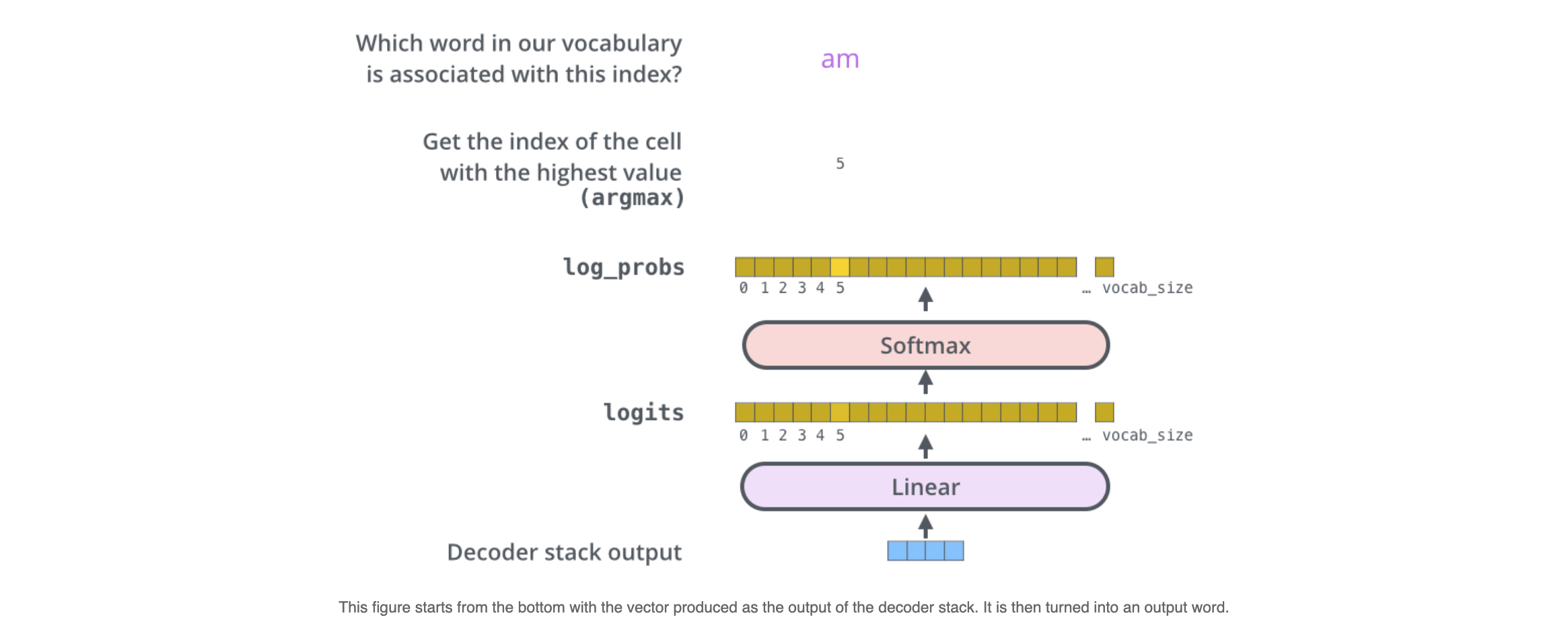
The output of the decoders is passed into a linear layer with softmax activation using which, the correct word is predicted.
Once the transformer predicts a word using forward propagation, the prediction is compared with the actual label using a loss function like cross-entropy and then all the trainable parameters are updated using back-propagation.
Well, this is one simplified way of understanding how learning happens in transformers. There are more variations like taking the complete output sentence for calculating the loss. To know more you can check out this amazing blog on Transformer by Jay Alammar.
With this, we have come to the end of this blog. Hope the read was pleasant. I would like to thank all the creators for creating the awesome content I referred to for writing this blog.
Reference links:
-
https://en.wikipedia.org/wiki/Transformer_(machine_learning_model)
-
https://medium.com/inside-machine-learning/what-is-a-transformer-d07dd1fbec04
Final note
Thank you for reading the blog. I hope it was useful for some of you aspiring to do projects or learn some new concepts in NLP.
In part 2/3 we will go through BERT (Bidirectional Encoder Representations from Transformers).
In part 3/3 we will go through a hands-on Kaggle challenge — Google QUEST Q&A Labeling to see Transformers in action (top 4.4% on the leaderboard).
Find me on LinkedIn: www.linkedin.com/in/sarthak-vajpayee
Peace! ☮